Conditional Formatting

Introduction

Conditional formatting in Excel is pretty simple. Most users are familiar with this feature off the Home tab. This approach allows you to format cells and control if the format is applied or not by filling a simple text box. For example if, in a column, a number is greater than 250 then format it with bold and Red.

In this post we are going to examine an innovative way to use Conditional Formatting. Suppose we have a 10 column list of transactions (or anything else) and we want to highlight the whole row based on a condition in one of the column. Is that possible? It’s actually pretty simple!

Below are the general steps. After you have considered them once or twice we will see a few examples.

Conditional formatting in a list

In an Excel list we want to highlight all rows where the region in column C is South. Below are the general steps for a fictitious list:

• Select the whole table (without the column headings). A quick way to do that is to select the first data entry in the list (upper left of the table) then press Ctrl+Shift+<Down Arrow> then <Right Arrow>.
• The whole data list is selected. Press Ctrl+<Backspace> to return at the top of the list.
• In the Home tab select Conditional Formatting then New Rules further down.
• In the Select a Rule Type list select the last entry, “Use a formula to determine which cells to format“.
• In the bottom half of the dialog box there is a textbox labeled “Format values where this formula is true“. This is the box we will focus on in this post.
• Type: =$D2=”South”
• Below click the Format button and, in the Fill tab, select a pale colour near the top of the colour palette. Then click OK to exit both dialog boxes.

The important feature above is the label “Format values where the formula is true“. This statement is the key to master this feature quickly and impress all your friends!

The formula in the box is one that returns True or False. If you’ve done a few IF() statements in the past you know exactly what this means. In a IF() formula the first argument is a conditional statement for the content of a cell. The second argument is evaluated when the condition results in a True. The third argument is evaluated when the condition is False.

When used in the context of Conditional Formatting, the format is applied if the condition is True otherwise not format is applied. Simple as that!

Remember!

The formula needs to evaluate the condition in the first row of the list!

Example of formulas to use with Conditional Formatting

Why do we need to use the a mixed reference?

You noticed that each reference use a mixed reference with the $ before the column. When a conditional formatting is applied in a list, it scans across every cells starting from the first row down to the last row.

However using the formula =$E2=”South” ensures that the criteria will always be compared with a cell in column E. Look at the example below. Cell E2 does not contain the entry South so Conditional Formatting ignores all cells in that row. However, in row 4 the entry in column E contains the entry South. In this case all cells in that row are formatted.

1st Example

The list does no have to start in row 1.

It is irrelevant where the list start since you have selected all the data (without the column headings).

Let’s look at a couple examples.

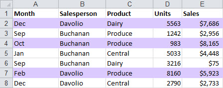
In the example below we want to highlight every rows where the Sales amount is greater or equal to $5,000. Since the Sales are in column E, we will use the formula: =$E2>=5000. All that is left to do is to highlight the rows with the colour of your choice.

2nd Example

In the next example, we use a formula having two conditions.
Below we want to highlight all rows where the product is Dairy and the date is in April. Since both condition needs to be met, we will use the expression: =AND($B2=”Dairy”, TEXT($F2,”mmm”)=”Apr”)

3rd Example

In the example above, if we had used the OR logical operator instead then all rows having either North or April or both would have been highlighted.

The next one is pretty cool! It highlight the largest value for each row. To achieve this, we use the MAX() function. Here’s how it works, the MAX() function returns the largest value in a row and compare that highest value to each amounts in that row. Logically, there has to be one (or more) value matching the highest value. When found, it is formatted.

4th Example

Finally, our last example uses a condition where the sum the two values in columns B and C is less than the value in cell G2. Here we use the formula: =$B2+$C2<=$G$2.

5th Example

Note in this example that we had to use an absolute reference for G2. Remember how Conditional Formatting scans a list? Every cells in the list (the one we’re interested are in columns B and C) are compared to the unique constant in G2. The amount 600 is used for every cells in the table (across & down). Thus we need to use he reference $G$2.

Why is this example so cool?

In our last example, changing the value in cell G2 will re-evaluate the conditional formatting rule. This will change the condition and a new set of rows will be highlighted!

Every example in this post use the same technique. They all use the option
“Use a formula to determine which cells to format“. Every formula is the type that return True or False. That’s the trick!

Now let’s Try It

Download a Zip file containing the Excel workbook you can use for the example above. Additionally, the workbook contains two more worksheets you can use to challenge yourself.

If you like this post please leave a short message below and tell your friends!

Daniel from ComboProjects